Chapter 2 Estimations

2.1 Statistical Inference

The process of making educated guess and conclusions regarding a population, using a sample of that population is called Statistical Inference.
Two important problems in statistical inference are estimation of parameters and tests of hypothesis
Estimation can be of the form of point estimation and interval estimation.

2.2 Point Estimation

Main Task

Assume that some characteristic of the elements in a population can be represented by a random variable $X$.
Assume that $X_1, X_2, \dots, X_n$ is a random sample from a density $f(x, \theta)$, where the form of the density is known but the parameter $\theta$ is unknown.
The objective is to construct good estimators for $\theta$ or its function $\tau (\theta)$ on the basis of the observed sample values $x_1, x_2, \dots, x_n$ of a random sample $X_1, X_2, \dots, X_n$ from $f(x, \theta)$.

Definition: Statistic

Suppose $X_1, X_2, \dots, X_n$ be $n$ observable random variables. Then, a known function $T=g(X_1, X_2, \dots, X_n)$ of observable random variables $X_1, X_2, \dots, X_n$ is called a statistic. A statistic is always a random variable.

Definition: Estimator

Suppose $X_1, X_2, \dots, X_n$ is a random sample from from a density $f(x, \theta)$ and it is desired to estimate $\theta$. Suppose $T=g(X_1, X_2, \dots, X_n)$ is a statistic that can be used to determine and approximate value for $\theta$. Then $T$ is called an estimator for $\theta$. An estimator is always a random variable.

Definition: Estimate

Suppose $T=g(X_1, X_2, \dots, X_n)$ be an estimator for $\theta$. Suppose that $x_1, x_2, \dots, x_n$ is a set of observed values of the random variable $X_1, X_2, \dots, X_n.$ Then the value $t=g(x_1, x_2, \dots, x_n)$ obtained by substituting the observed values in the estimator is called an estimate for $\theta$.

Therefore the estimator stands for the function of the sample, and the word estimate stands for the realized value of that function.
Notation: An estimator of $\theta$ is denoted by $\hat{\theta}$. An estimate of $\theta$ is also denoted by $\hat{\theta}$. The difference between the two should be understood based on the context.

Parameter	Estimator: Using random sample ($X_1, X_2, \dots, X_n$)	Estimate 1: Using observed sample ($1,4,2,3,4$)	Estimate 2: Using observed sample ($4,2,2,6,3$)
$\mu$	$\hat{\mu}=\bar{X}$	$\hat{\mu}=$	$\hat{\mu}=$
$\sigma^2$	$\hat{\sigma^2}=S^2$	$\hat{\sigma^2}=$	$\hat{\sigma^2}=$

2.2.1 Methods of finding point estimators

In some cases there will be an obvious or natural candidate for a point estimator of a particular parameter.
For example, the sample mean is a good point estimator of the population mean
However, in more complicated models we need a methodical way of estimating parameters.
There are different methods of finding point estimators
- Method of Moments
- Maximum Likelihood Estimators (MLE)
- Method of Least Squares
- Bayes Estimators
- The EM Algorithm
However, these techniques do not carry any guarantees with them
The point estimators that they yeild still must be evaluated before their worth is established

2.2.1.1 Method of Moments

Let $X_1, X_2, \dots X_n$ be a random sample from a population with pdf or pmf $f(x; \theta),$ where $\theta = (\theta_1, \theta_2, \dots, \theta_k)$ and $k\geq 1$.
Sample moments $m^\prime$ and population moments $\mu^\prime$ are defined as follows

Sample moment	Population moment
$m_1^\prime= \frac{1}{n}\sum_{i=1}^nX_i$	$\mu_1=E(X)$
$m_2^\prime= \frac{1}{n}\sum_{i=1}^nX_i^2$	$\mu_2=E(X^2)$
$\dots$	$\dots$
$m_k^\prime= \frac{1}{n}\sum_{i=1}^nX_i^k$	$\mu_k=E(X^k)$

Each $\mu_j^\prime$ is a function $\theta,$ i.e. $\mu_j^\prime= \mu_j^\prime(\theta_1, \theta_2, \dots, \theta_k)$ for $j=1,2,\dots, k.$

Method of Moments Estimators (MME)

We first equate the first $k$ sample moments to the corresponding $k$ population moments,

\[m_1^\prime = \mu_1^\prime,\] \[m_2^\prime = \mu_2^\prime,\] \[\dots\] \[m_k^\prime = \mu_k^\prime,\]

Then we solve the resulting systems of simultaneous equations for $\hat{\theta_1}, \hat{\theta_2}, \dots, \hat{\theta_k}$

Remarks on Method of Moments Estimators

Very easy to compute
Always give an estimator to start with
Generally consistent (Since sample moments are consistent for population moments)
Not necessarily the best or most efficient estimators

2.2.1.2 Maximum Likelihood Estimators (MLE)

Example

The number of orders per day coming to a certain company seems to have a Poisson distribution with parameter $\lambda$.

The number of orders received during 10 randomly selected days are as follows: $12,14,15,12,13,10,11,15,10,6$

Derive an expression for the $P(X_1=12, \; X_2 = 14, \dots, X_{10} = 10)$ as a function of $\lambda.$

Find the joint probability of the data

$Probability of the sample is maximum when $\lambda = 11.8$$

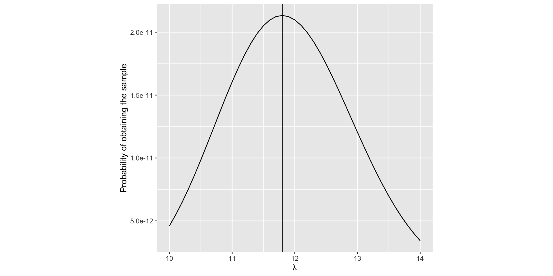
Figure 2.1: Probability of the sample is maximum when $\lambda = 11.8$

When it is viewed as a function of $\lambda$, it is called the likelihood function of $\lambda$ for the available data
The likelihood for the data is maximum when $\lambda = 11.8.$
Since these data have already occurred, it is very likely that the data have arisen from a Poisson distribution with $\lambda =11.8$.
This estimate for $\lambda$ is called the maximum likelihood estimate
In order to define maximum-likelihood estimators, we shall first define the likelihood function.

Definition: Likelihood function

Let $x_1,x_2, \dots, x_n$ be a set of observations of random variables $X_1, X_2, \dots, X_n$ with the joint density of $n$ random variables, say $f_{X_1, X_2, \dots, X_n}(x_1,x_2, \dots, x_n;\; \theta)$. This joint density function, which is considered to be a function of $\theta$ is called the likelihood function of $\theta$ for the set of observations (sample) $x_1,x_2, \dots, x_n.$

In particular, if $x_1,x_2, \dots, x_n$ is a random sample from the density $f(x; \theta)$, then the likelihood function is $f(x_1; \theta)f(x_2; \theta) \dots f(x_n; \theta).$

Notation

We use the notation $L(\theta;\;x_1,x_2, \dots, x_n)$ for the likelihood function, in order to remind ourselves to think of the likelihood function as a function of $\theta.$

Likelihood function is seen as a function of $\theta$ rather than $x$
Likelihood can be viewed as the degree of plausibility.
An estimate of $\theta$ may be obtained by choosing the most plausible value, i.e., where the likelihood function is maximized.

Definition: Maximum Likelihood Estimator

Let $L(\theta)=L(\theta;\;x_1,x_2, \dots, x_n)$ be the likelihood function of $\theta$ for the sample $x_1,x_2, \dots, x_n.$ Suppose $L(\theta)$ has its maximum when $\theta = \hat{\theta}.$

Then $\hat{\theta}$ is called the Maximum likelihood estimate of $\theta$.

The corresponding estimator is called the Maximum likelihood estimator of $\theta$.

Many likelihood functions satisfy regularity conditions; so the maximum likelihood estimator is the solution of the equation \[\frac{dL(\theta)}{d\theta} = 0\]

Log-likelihood function

Let \[l(\theta) = ln[L(\theta)].\]

Then, $l(\theta)$ is called the log-likelihood function.

Both $L(\theta)$ and $l(\theta)$ have their maxima at the same value of $\theta$.
It is sometimes easier tot find the maximum of the logarithm of the likelihood and thereby simplify the calculations in finding the maximum likelihood estimate.

Invariance Property of MLE’s

If $\hat{\theta}$ is the MLE of $\theta$, then for any function $\tau(\theta),$ the MLE of $\tau(\theta)$ is $\tau(\hat{\theta}).$

2.2.2 Desirable properties of point estimators

We discussed several methods of obtaining point estimators.
It is possible that different methods of finding estimators will lead to same estimator or different estimators.
In this section we discuss certain properties, which an estimator may or may not posses, that will guide us in deciding whether one estimator is better than another.

2.2.2.1 Unbiasedness

Definition: Unbiased estimator

An estimator $\hat{\theta}$ $(=t(X_1, X_2, \dots, X_n))$ is defined to be an unbiased estimator of $\theta$ if and only if \[E(\hat{\theta}) = \theta\]

The difference $E(\hat{\theta}) -\theta$ is called as the bias of $\hat{\theta}$ and denoted by \[Bias(\hat{\theta}) = E(\hat{\theta}) - \theta \]
An estimator whose bias is equal to 0 is called unbiased.

2.2.3 Consistency

Mean-Squared Error

The mean-squared error is a measure of goodness or closeness of an estimator to the target.

Definition: Mean-squared Error (MSE)

The mean-squared error of an estimator $\hat{\theta}$ of $\theta$ is defined as \[MSE(\hat{\theta})= E\left[(\hat{\theta} - \theta)^2 \right]\]

The MSE measures the average squared difference between $\hat{\theta}$ and $\theta$.
The MSE is a function of $\theta$ and has the interpretation

\[MSE(\hat{\theta})= Var(\hat{\theta})+ \left[Bias(\hat{\theta}) \right]^2\]

Therefore the MSE incorporates two components, one measuring the variability of the estimator (precision) and the other measuring its bias (accuracy).
Small value of MSE implies small combined variance and bias.
If $\hat{\theta}$ is unbiased, then \[MSE(\hat{\theta})= Var(\hat{\theta})\]
The positive square root of MSE is known as the root mean squared error \[RMSE(\hat{\theta})= \sqrt{MSE(\hat{\theta})}\]

Consistency

Estimator $\hat{\theta}$ is said to be consistent for $\theta$ if $MSE(\hat{\theta})$ approaches zero as the sample size $n$ approaches $\infty$.

\[lim_{n\rightarrow \infty}E\left[(\hat{\theta} - \theta)^2 \right]=0\]

Mean-squared error consistency implies that the bias and the variance both approach to zero as $n$ approaches $\infty.$

2.3 Interval Estimation

Under point estimation of a parameter $\theta$, the inference is a guess of a single value as the value of $\theta$.
Instead of making the inference of estimating the true value of the parameter to be a point, under interval estimation we make the inference of estimating that the true value of the parameter is contained in some interval.

2.3.1 What is gained by using an Interval Estimator?

Example

For a sample $X_1, X_2, X_3, X_4$ from a $N(\mu, 1),$ an interval estimator of $\mu$ is $[\bar{X}-1, \bar{X}+1].$
This means that we will assert that $\mu$ is in this interval.
In the previous section (Point estimation) we estimated $\mu$ with $\bar{X}.$
But now we have the less precise estimator $[\bar{X}-1, \bar{X}+1]$.
Under interval estimation, by giving up some precision in our estimate (or assertion about $\mu$), we try to gain some confidence , or assurance that our assertion is correct.

Explanation

When we estimate $\mu$ by $\bar{X},$ the probability that the estimator exactly equaled the value of the parameter being estimated is zero (Why? the probability that a continuous random variable equals any value is 0), i.e. $P(\bar{X}=\mu) = 0.$
However, with an interval estimator, we have a positive probability of being correct.
The probability that $\mu$ is covered by the interval $[\bar{X}-1, \bar{X}+1]$ can be calculated as \[P(\mu \in [\bar{X}-1, \bar{X}+1])= P(\bar{X}-1 \leq \mu\leq \bar{X}+1)\] \[ = P(-1 \leq \bar{X} - \mu\leq 1)\] \[ = P(- 2\leq \frac{\bar{X} - \mu}{\sqrt{1/4}}\leq 2)\] \[ = P(- 2\leq Z\leq 2)\;\;\; \left(\frac{\bar{X} - \mu}{\sqrt{1/4}} \text{ is standard normal }\right)\] \[=0.9544.\]
Therefore now we have over 95% chance of covering the unknown parameter with the interval estimator.
By moving for a point to an interval we have scarified some precision in our estimate. But it has resulted in increased confidence that our assertion is correct.
The purpose of using an interval estimator rather than a point estimator is to have some guarantee of capturing the parameter of interest.

2.3.2 Definition of confidence interval

Definition

Let $X_1, X_2, \dots, X_n$ be a random sample from a distribution with parameter $\theta.$ Let $T_1 = g(X_1, X_2, \dots, X_n),$ and $T_2 = h(X_1, X_2, \dots, X_n)$ be two statistics satisfying $T_1 \leq T_2$ for which $P(T_1 < \theta < T_2)= \gamma,$ where $\gamma$ does not depend on $\theta$. Then, the random interval $(T_1, T_2)$ is called a $100\gamma$ percent confidence interval for $\theta$; $\gamma$ is called the confidence coefficient; and $T_1$ $T_2$ are called the lower and upper confidence limits, respectively, for $\theta.$

Suppose that $x_1, x_2, \dots, x_n$ is a realization of $X_1, X_2, \dots, X_n$ and let $t_1 = g(x_1, x_2, \dots, x_n),$ and $t_2 = h(x_1, x_2, \dots, x_n)$. Then the numerical interval $(t_1, t_2)$ is also called a $100\gamma$ percent confidence interval for $\theta$.

2.3.3 Interpretation of confidence intervals

Consider the probability statement $P(\bar{X}-1.18 \leq \mu\leq \bar{X}+1.18) =0.95.$
The above probability statement implies that the random interval $(\bar{X}-1.18, \bar{X}+1.18)$ includes the unknown true mean $\mu$ with probability 0.95.

2.3.4 Methods of finding interval estimators

2.3.4.1 Pivotal Quantity Method

Definition: Pivotal Quantity

Let $X_1, X_2,\dots, X_n$ be a random sample from the density $f(.;\theta).$ Let $Q=q(X_1, X_2,\dots, X_n; \theta)$; that is, let $Q$ be a function of $X_1, X_2,\dots, X_n$ and $\theta$. If $Q$ has a distribution that does not depend on $\theta$, then $Q$ is defined to be a pivotal quantity

Pivotal Quantity method

If $Q=q(X_1, X_2,\dots, X_n; \theta)$ is a pivotal quantity and has a probability density function, then for any fixed $0<\gamma<1$ there will exist $q_1$ and $q_2$ depending on $\gamma$ such that $P[q_1<Q<q_2]=\gamma.$ Now, if for each possible sample value $(x_1, x_2, \dots, x_n),$ $q_1< q(x_1, x_2,\dots, x_n; \theta)< q_2$ if and only if $t_1(x_1, x_2,\dots, x_n)<\tau(\theta)<t_2(x_1, x_2,\dots, x_n)$ for functions $t_1$ and $t_2$ (not depending on $\theta$), then $(T_1, T_2)$ is a $100\gamma$ percent confidence interval for $\tau(\theta),$ where $T_1=t_1(X_1, X_2,\dots, X_n)$ and $T_2=t_2(X_1, X_2,\dots, X_n)$.

2.3.5 Methods of evaluating interval estimators

Coverage probability
Size (expected length)

Tutorial

Let $X_1, X_2, \dots, X_n \sim iid\;\; N(\mu, \sigma^2),$ both $\mu$ and $\sigma^2$ unknown. Derive a method of moment estimators for $\mu$ and $\sigma$.
Let $X_1, X_2, \dots, X_n \sim iid\;\; Bin(n,\theta),$ both $n$ and $\theta$ unknown. Derive a method of moment estimators for $n$ and $\theta$.
Let $X_1, X_2, \dots, X_n \sim iid\;\; Unif(\theta_1,\theta_2),$ where $\theta_1<\theta_2$, both unknown. Derive a method of moment estimators for $\theta_1$ and $\theta_2$.
Let $X_1, X_2, \dots, X_n \sim Poisson(\lambda).$ Derive a method of moment estimators for $\lambda$.
Let $X_1, X_2, \dots, X_n \sim iid\;\; Gamma(\alpha,\beta),$ both $\alpha$ and $\beta$ unknown. Derive a method of moment estimators for $\alpha$ and $\beta$.

The survival time (in weeks) of 20 randomly selected male mouse exposed to 240 units of certain type of radiation are given below.

$152, 115, 109, 94, 88, 137, 152, 77, 160, 165, 125, 40, 128, 123, 136, 101, 62, 153, 83, 69$

It is believed that the survival times have a gamma distribution. Estimate the corresponding parameters.

Let $x_1, x_2, \dots, x_n$ be $n$ random measurements of random variable $X$ with the density function \[f_X(x;\lambda)= \lambda x^{\lambda-1},\;\; 0<x<1, \;\; \lambda>0\] Derive a method of moment estimator for $\lambda$.

Let $x_1, x_2, \dots, x_n$ be a random sample of size $n$ from a Poisson distribution with parameter $\lambda$. Derive the maximum likelihood estimator of $\lambda$.
Let $x_1, x_2, \dots, x_n$ be a random sample of size $n$ from a normal distribution with mean $\mu$ and variance $\sigma^2$. Derive the maximum likelihood estimators of $\mu$ and $\sigma^2$.

Let $X_1, X_2, \dots, X_n \sim iid \; Poisson (\lambda)$. Find the MLE of $P(X\leq 1)$

Let $X_1, X_2, \dots, X_n \sim iid \; N (\mu, \sigma^2)$. Find the MLE of $\mu/\sigma$.

Let $X_1, X_2, \dots, X_n$ be a random sample from an exponential distribution with the density function \[f_X(x;\lambda)= \lambda e^{-\lambda x},\;\; x>0\]. Is the maximum likelihood estimators of $\lambda$ unbiased?

Let $X_1, X_2, \dots, X_n$ be a random sample of size $n$ from a distribution with mean $\mu$ and variance $\sigma^2$. Show that $\bar{X}$ and $S^2 = \frac{\sum_{i=1}^n(X_i-\bar{X})^2}{n-1}$ are unbiased estimators of $\mu$ and $\sigma^2$, respectively.

Let $x_1, x_2, \dots, x_n$ be a random sample of size $n$ from a normal distribution with mean $\mu$ and variance $\sigma^2$. Consider the maximum likelihood estimators of $\sigma^2$. Show the estimator $\hat{\sigma^2} = \frac{\sum_{i=1}^n(X_i-\bar{X})^2}{n}$ is biased for $\sigma^2$, but it has a smaller MSE than $S^2 = \frac{\sum_{i=1}^n(X_i-\bar{X})^2}{n-1}$.

Let $X_1, X_2, \dots, X_n$ be a random sample from some distribution and $E(X) = \mu$. Show that $\bar{X}$ is a better estimator than $X_1$ and $\frac{X_1+X_2}{2}$ for $\mu$ in terms of MSE.

Let $X_1, X_2, \dots, X_n$ be a random sample from a $N(\mu, \sigma^2).$ Let $\bar{X}= \frac{\sum_{i=1}^nX_i}{n}$ and $T=\frac{\sum_{i=1}^n(X_i-\bar{X})^2}{n}$. Show that $\bar{X}$ is consistent for $\mu$ and $T$ is consistent for $\sigma^2.$

Let $X_1, X_2, \dots, X_n$ be a random sample from a $N(\mu,9).$ Find a 95% confidence interval for $\mu$.

Let $X_1, X_2, \dots, X_n$ be a random sample from a $N(\mu,\sigma^2),$ both $\mu$ and $\sigma$ are unknown. Construct a $100(1-\alpha)\%$ $(0<\alpha<1)$ confidence interval for $\mu$.

Let $X_1, X_2, \dots, X_n$ be a random sample from a $N(\mu,\sigma^2),.$ Construct a $100(1-\alpha)\%$ $(0<\alpha<1)$ confidence interval for $\sigma^2$.

Parameter	Estimator: Using random sample (\(X_1, X_2, \dots, X_n\))	Estimate 1: Using observed sample (\(1,4,2,3,4\))	Estimate 2: Using observed sample (\(4,2,2,6,3\))
\(\mu\)	\(\hat{\mu}=\bar{X}\)	\(\hat{\mu}=\)	\(\hat{\mu}=\)
\(\sigma^2\)	\(\hat{\sigma^2}=S^2\)	\(\hat{\sigma^2}=\)	\(\hat{\sigma^2}=\)

Sample moment	Population moment
\(m_1^\prime= \frac{1}{n}\sum_{i=1}^nX_i\)	\(\mu_1=E(X)\)
\(m_2^\prime= \frac{1}{n}\sum_{i=1}^nX_i^2\)	\(\mu_2=E(X^2)\)
\(\dots\)	\(\dots\)
\(m_k^\prime= \frac{1}{n}\sum_{i=1}^nX_i^k\)	\(\mu_k=E(X^k)\)