Chapter 4 Contingency Tables

In Chapters 2 (Estimations) and 3 (Hypothesis Testing) we briefly discussed about the chi-square distribution in the construction of confidence intervals for and the testing of hypotheses concerning a population variance.
Chi-square distribution, which is one of the most widely used distributions in statistical applications, has many other uses.
The chi-square distribution is the most frequently employed statistical technique for the analysis of categorical data.

4.1 Types of chi-square tests

Chi square test has two cases:

Chi-square goodness of fit test
Chi-square test of independence. This is also known as contingency analysis.

In this chapter our focus is on chi-square test of independence

4.2 Contingency analysis: Chi-square test of independence

Chi-square test of independence is a statistical test used to analyse the frequencies of two variables with multiple categories to determine whether the two variables are independent.
For example, a software developer might want to determine whether the user ranking of user-friendliness (Very Satisfied = 5, Satisfied = 4, Neutral = 3, Dissatisfied = 2, Very Dissatisfied = 1) of the new software product is independent of the user’s education level.

A market researcher might want to determine whether the type of online communication platforms (eg:Slack, Zula, ezTalks, HipChat, Yammar) preferred by a user is independent of the user’s age.
A software project manager might want to know whether customer overall satisfaction (Very Satisfied = 5, Satisfied = 4, Neutral = 3, Dissatisfied = 2, Very Dissatisfied = 1 is independent of the experience of the developer (less than 1 year, 1-5 years, more than 5 years)

Example

A software company is planning to develop a new taxi booking and trip scheduling platform that facilitates a real time connection between the commuter and the taxi driver, enabling mutual engagement for the receipt and delivery of a service. Prior to development, the management wants to identify the strength and weakness of the existing services as they may be their potential competitors. Suppose the project manager is interested in determining whether the type of taxi service preferred by a commuter is independent of the commuter’s age.

On a questionnaire, the following two questions might be used to measure these aspects.

What is your most preferred taxi booking and trip scheduling platform?

Uber
PickMe

Select your age category?

\(< 30\) years
\(30-50\) years
\(>50\) years

4.2.1 Contingency table

Let the number of responses received were 100.
Now the analyst can tally the frequencies of responses to these two questions into a two-way table called contingency table

Contingency table

	Most preferred taxi booking and trip scheduling platform
Age	Uber	PickMe	Total
\(< 30\) years	32	25	57
\(30-50\) years	18	5	23
\(> 50\) years	17	3	20
Total	67	33	100

Because the chi-square test of independence uses a contingency table, this test is sometimes referred to as contingency analysis

Contingency table

	Variable 2
Variable 1	F	G	H	Total
A			\(o_{13}\)	\(n_A\)
B				\(n_B\)
C				\(n_C\)
D				\(n_D\)
E				\(n_E\)
Total	\(n_F\)	\(n_G\)	\(n_H\)

The observed frequency for for each cell is denoted as \(o_{ij},\) where \(i\) is the row and \(j\) is the column.
The expected frequencies are denoted in a similar manner.
If two variables are independent, they are not related.
In a sense, the chi-square test of independence is a test of whether the variables are related.
The null hypothesis for a chi-square test of independence is that the two variables are independent (not related).
If the null hypothesis is rejected, the conclusion is that the two variables are not independent and are related.
In general, if the two variables are independent, the expected frequency values of each call can be determined by

\[e_{ij} = \frac{n_in_j}{N}\]

where:

\(i =\) the row
\(j =\) the column
\(n_i =\) the total of row \(i\)
\(n_j =\) the total of column \(j\)
\(N =\) the total of all frequencies

Using these expected frequency values and the observed frequency value, we can compute a chi-square test of independence to determine whether the variables are independent.

4.2.2 Chi-square test of independence

\[\chi^2 =\sum_r\sum_c \frac{(f_0-f_e)^2}{f_e}\]

where - \(df = (r-1)(c-1)\) - \(r=\) number of rows - \(c=\) number few columns - \(\sum_r=\) sum over row - \(\sum_c=\) sum over column

The null hypothesis for a chi-square test of independence is that the two variables are independent.
The alternative hypothesis for a chi-square test of independence is that the two variables are not independent
This test is one one-tailed.

The degrees of freedom are \((r-1)(c-1)\)

Caution

In chi-square test of independence, small expected frequencies can lead to inordinately large chi-square values.
Therefore, contingency tables should not be used with expected cell values of less than 5.
One way to avoid small expected values is to combine columns or rows whenever possible and whenever doing so make sense.

Example contd…

Suppose the project manager is interested in determining whether the type of taxi service preferred by a commuter is independent of the commuter’s age. He conducted a small survey to determine. He received 100 responses. The resulting \(3\times2\) contingency table is given below. Using \(\alpha =0.05,\) perform the chi-square test of independence to determine whether preferred mode is independent of age.

	Most preferred taxi booking and trip scheduling platform
Age	Uber	PickMe	Total
\(< 30\) years	32	25	57
\(30-50\) years	18	5	23
\(> 50\) years	17	3	20
Total	67	33	100

4.3 Chi-square test of independence with R

Let us now see how to perform the Chi-square test of independence using R programming language

Following is the observed table.

observed_table <- matrix(c(32, 25, 18, 5, 17, 3), nrow = 3, ncol = 2, byrow = T)
rownames(observed_table) <- c('<30', '30-50', '>50')
colnames(observed_table) <- c('Uber', 'PickMe')
observed_table

##       Uber PickMe
## <30     32     25
## 30-50   18      5
## >50     17      3

addmargins(observed_table)

##       Uber PickMe Sum
## <30     32     25  57
## 30-50   18      5  23
## >50     17      3  20
## Sum     67     33 100

In order to perform the test, we need to apply the chisq.test() function to the observed table.

output <- chisq.test(observed_table)
output

## 
##  Pearson's Chi-squared test
## 
## data:  observed_table
## X-squared = 7.2902, df = 2, p-value = 0.02612

From the above result, we can see that p-value is less than the significance level (0.05). Therefore, we can reject the null hypothesis and conclude that the two variables (age & taxi preference) are not independent
If we want to see the expected table, we can also do that.

output$expected

##        Uber PickMe
## <30   38.19  18.81
## 30-50 15.41   7.59
## >50   13.40   6.60

Visualizing data of Contingency Table with ggplot2 (Side By Side Bar Graph)

library(tidyverse)

table2 <- observed_table %>%
  as.data.frame() %>%
  rownames_to_column() %>%
  gather(Column, Value, -rowname)

colnames(table2) <- c('Age', 'Mode', "Count")
table2

##     Age   Mode Count
## 1   <30   Uber    32
## 2 30-50   Uber    18
## 3   >50   Uber    17
## 4   <30 PickMe    25
## 5 30-50 PickMe     5
## 6   >50 PickMe     3

ggplot(data = table2, aes(x = Age, y = Count, fill = Mode)) + 
  geom_bar(stat = "identity", position = "dodge") +
  scale_fill_grey()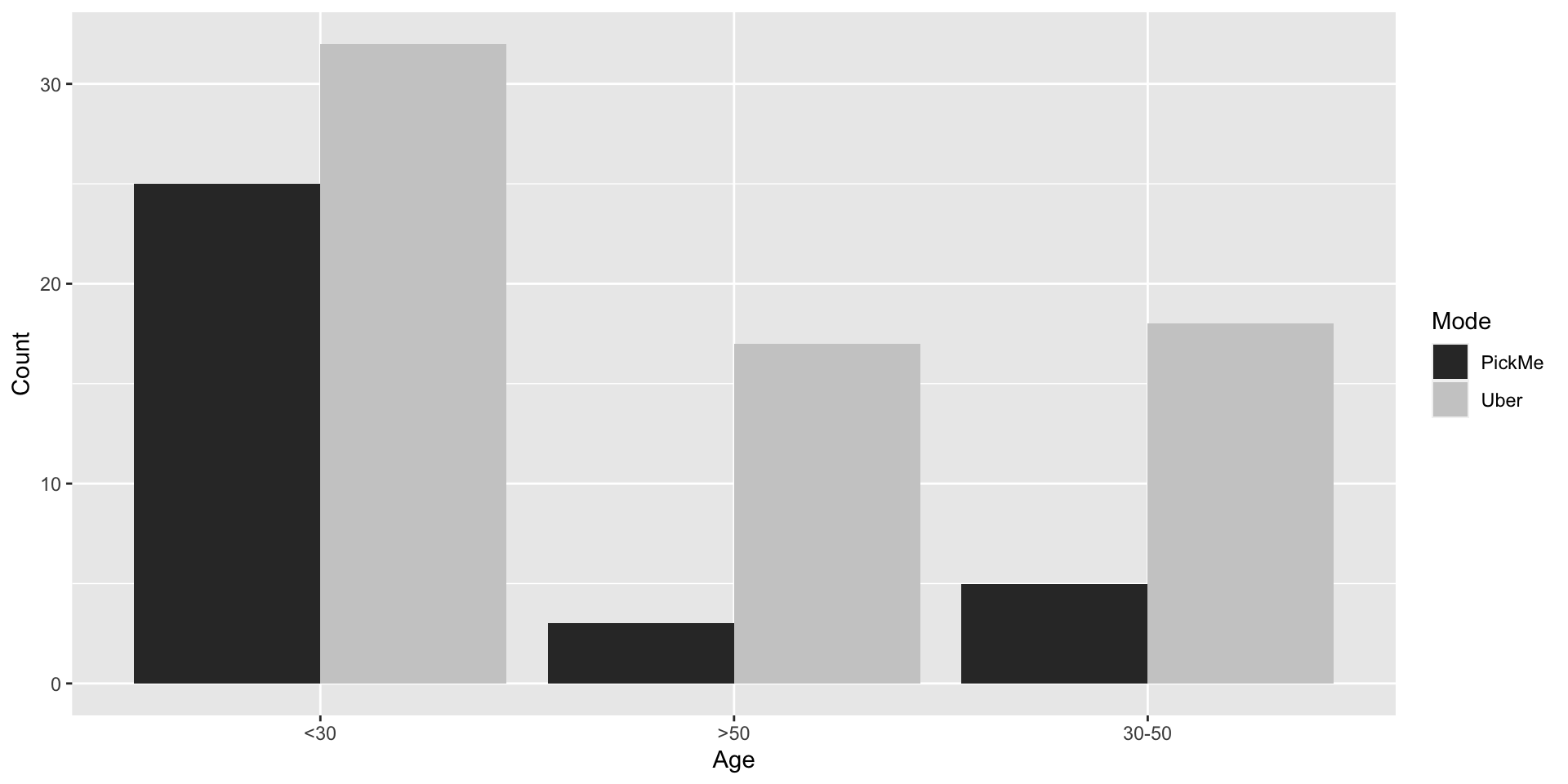

References

Black, K., Asafu-Adjaye, J., Khan, N., Perera, N., Edwards, P., & Harris, M. (2007). Australasian business statistics. John Wiley & Sons.
Daniel, W. W., & Cross, C. L. (2018). Biostatistics: a foundation for analysis in the health sciences. Wiley.

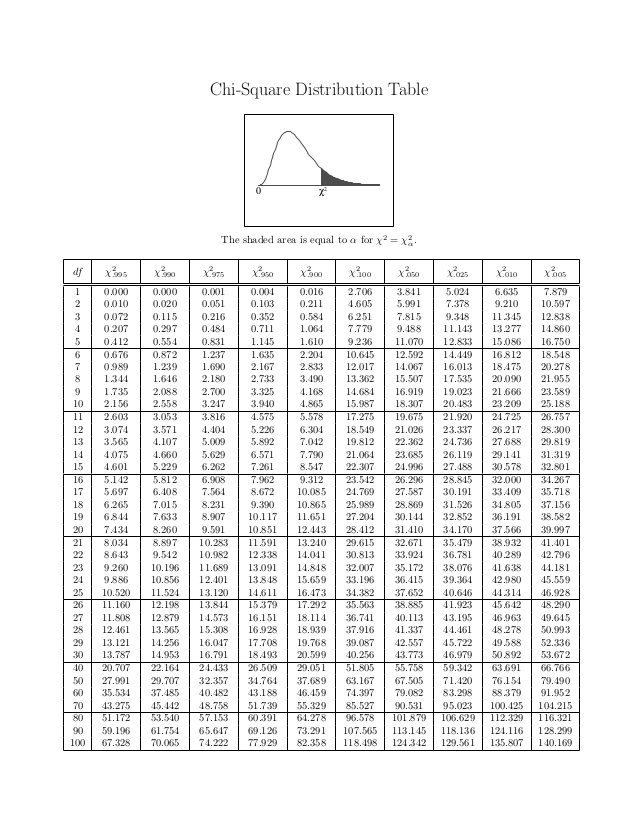
Critical values from the chi-square distribution

Tutorial

A company maintain an online food ordering service. Suppose market researcher wants to know whether the type of beverage ordered with lunch is independent of the food delivery zone (area). A random sample of 309 lunch customers is selected, resulting in the following contingency table of observed values. Use \(\alpha = 0.01\) to determine whether the two variables are independent.

	Preferred beverage
Zone	Fresh Fruit Juice	Soft drink	Other
Zone 1	26	95	18
Zone 2	41	40	20
Zone 3	24	13	32

A computer manufacturer is considering sourcing supplies of an electrical component from four different manufacturers. The director of purchasing asked for samples of 95 from each manufacturer. The numbers of acceptable and unacceptable components from each manufacturer are shown in the following table. Determine whether the quality of the component depends on the type of manufacturer. Let \(\alpha =0.05\)

	Manufacturer
Quality	A	B	C	D	Total
Unacceptable	12	8	5	11	36
Acceptable	83	87	90	84	344
Total	95	95	95	95	380

An apparel & clothing market research company conducted a survey in 2019 on social media usage of university students. The frequencies for most frequently used social media platform by male and female students (in thousands) are presented in the following contingency table. Using \(\alpha =0.01\), test the hypothesis that social media preference is independent of gender.

	Social media platform
Gender	Facebook	Instagram	Twitter	Total
Male	687	327	82	1096
Female	658	304	101	1063
Total	1345	631	183	2159

Use R to make a decision for Question 1
Use R to make a decision for Question 2
Use R to make a decision for Question 3