2  R Programming Basics

• R has two main parts: data structures and functions.

  • Data structures help store and organize data so it can be used efficiently.

 income <- c(1000, 4000, 3400, 9700, 9800)
 income

[1] 1000 4000 3400 9700 9800

-   Functions tell R what to do.

mean(income)

[1] 5580

summary(income)

   Min. 1st Qu.  Median    Mean 3rd Qu.    Max. 
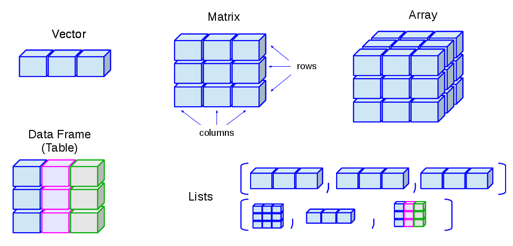
   1000    3400    4000    5580    9700    9800 

2.1 Data structures

• R’s basic data structures can be grouped by:

  • Their dimensions (1D, 2D, or multi-dimensional).
  • Whether they store one type of data (homogeneous) or different types of data (heterogeneous).

• This gives us five common data structures in R:

  • Homogeneous (same type of data): Vectors, Matrices, Arrays
  • Heterogeneous (different types of data): Data Frames, Lists

Data Structure Types. Image Source: http://venus.ifca.unican.es/Rintro/dataStruct.html

• Among these, vectors and data frames are the most commonly used data structures in practical applications.

2.1.1 Vectors

Creating vectors

Syntax

vector_name <- c(element1, element2, element3)

Example

x <- c(5, 6, 3, 1, 100)
x

[1]   5   6   3   1 100

Combine two vectors

p <- c(1, 2, 3)
p

[1] 1 2 3

q <- c(10, 20, 30)
q

[1] 10 20 30

r <- c(p, q)
r

[1]  1  2  3 10 20 30

Vector with charactor elements

countries <- c("Sri Lanka", "Afghanistan", "Bangladesh", "Bhutan", "India", "Iran", "Maldives", "Nepal", "Pakistan")

countries

[1] "Sri Lanka"   "Afghanistan" "Bangladesh"  "Bhutan"      "India"      
[6] "Iran"        "Maldives"    "Nepal"       "Pakistan"   

Logical vector

result <- c(TRUE, FALSE, FALSE, TRUE, FALSE)
result

[1]  TRUE FALSE FALSE  TRUE FALSE

Simplifying vector creation

• rep is a function in R that repeats the values in a vector

id <- 1:10
id

 [1]  1  2  3  4  5  6  7  8  9 10

treatment <- rep(1:3, each=2)
treatment

[1] 1 1 2 2 3 3

Vector operations

x <- c(1, 2, 3)
y <- c(10, 20, 30)
x+y

[1] 11 22 33

p <- c(100, 1000)
x+p

Warning in x + p: longer object length is not a multiple of shorter object
length

[1]  101 1002  103

2.2 Data Frames

Required R package to deal with data frames

library(tidyverse)

── Attaching core tidyverse packages ──────────────────────── tidyverse 2.0.0 ──
✔ dplyr     1.1.4     ✔ readr     2.1.5
✔ forcats   1.0.0     ✔ stringr   1.5.1
✔ ggplot2   3.5.1     ✔ tibble    3.2.1
✔ lubridate 1.9.3     ✔ tidyr     1.3.1
✔ purrr     1.0.2     
── Conflicts ────────────────────────────────────────── tidyverse_conflicts() ──
✖ dplyr::filter() masks stats::filter()
✖ dplyr::lag()    masks stats::lag()
ℹ Use the conflicted package (<http://conflicted.r-lib.org/>) to force all conflicts to become errors

Create a tibble

• A tibble is an improved version of a traditional data frame in R, designed to be more user-friendly and consistent.

• It is part of the tidyverse package and makes it easier to view and analyze data, especially when working with large datasets.

Lets consider the following example

GDP per capita (current US$) - South Asia

Data Source : https://data.worldbank.org/

Country	Most Recent Year	Most Recent Value
Afghanistan	2023	415.7
Bangladesh	2023	2,551.0
Bhutan	2023	NA
India	2023	2,480.8
Maldives	2023	12,530.4
Nepal	2023	1,377.6
Pakistan	2023	1,365.3
Sri Lanka	2023	3,828.0

country <- c("Afghanistan", "Bangladesh", "Bhutan", "India", "Maldives",
             "Nepal", "Pakistan", "Sri Lanka")
year <- c(rep(2023,8))
value <- c(415.7, 2551.0, NA, 2480.8, 12530.4, 1377.6, 1365.3, 3828.0)

final <- tibble(Country = country, Recent_Year = year, Value = value )
final

# A tibble: 8 × 3
  Country     Recent_Year  Value
  <chr>             <dbl>  <dbl>
1 Afghanistan        2023   416.
2 Bangladesh         2023  2551 
3 Bhutan             2023    NA 
4 India              2023  2481.
5 Maldives           2023 12530.
6 Nepal              2023  1378.
7 Pakistan           2023  1365.
8 Sri Lanka          2023  3828 

2.3 Functions in R

• In R, functions are blocks of code that perform specific tasks.

• They take input values (called arguments), process them, and return an output.

• Functions help automate repetitive tasks and make code more efficient.

• There are two main types of functions in R:

  • Built-in functions – Predefined in R (e.g., mean(), sum(), rep()).

summary(final$Value)

   Min. 1st Qu.  Median    Mean 3rd Qu.    Max.    NA's 
  415.7  1371.5  2480.8  3507.0  3189.5 12530.4       1 

- User-defined functions – Created by users for specific needs using function().

2.4 Subsetting

final

# A tibble: 8 × 3
  Country     Recent_Year  Value
  <chr>             <dbl>  <dbl>
1 Afghanistan        2023   416.
2 Bangladesh         2023  2551 
3 Bhutan             2023    NA 
4 India              2023  2481.
5 Maldives           2023 12530.
6 Nepal              2023  1378.
7 Pakistan           2023  1365.
8 Sri Lanka          2023  3828 

final[1, 1]

# A tibble: 1 × 1
  Country    
  <chr>      
1 Afghanistan

final[, 1]

# A tibble: 8 × 1
  Country    
  <chr>      
1 Afghanistan
2 Bangladesh 
3 Bhutan     
4 India      
5 Maldives   
6 Nepal      
7 Pakistan   
8 Sri Lanka  

final[1, ]

# A tibble: 1 × 3
  Country     Recent_Year Value
  <chr>             <dbl> <dbl>
1 Afghanistan        2023  416.

final$Country

[1] "Afghanistan" "Bangladesh"  "Bhutan"      "India"       "Maldives"   
[6] "Nepal"       "Pakistan"    "Sri Lanka"  

2.5 Help file for Built-in functions

• To access the help file for a built-in function in R, you can use either ? or the help() function.

• Running either of these commands will open the help page for the specified function.

= For example, using ?summary or help(summary) will display the help file for the summary function, which is part of the base R package.

?summary

# or 

help(summary)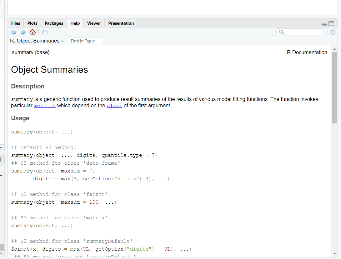

Help Page

2.6 Commenting

mean(final$Value) # Calculate the average GDP value

[1] NA

When you go to the help page for the mean() function, you’ll find that by default, the na.rm argument is set to FALSE. This means that if the data contains missing values (NA), they will be included in the calculation, and the result will also be NA. To calculate the mean while ignoring missing values, you should set na.rm = TRUE.

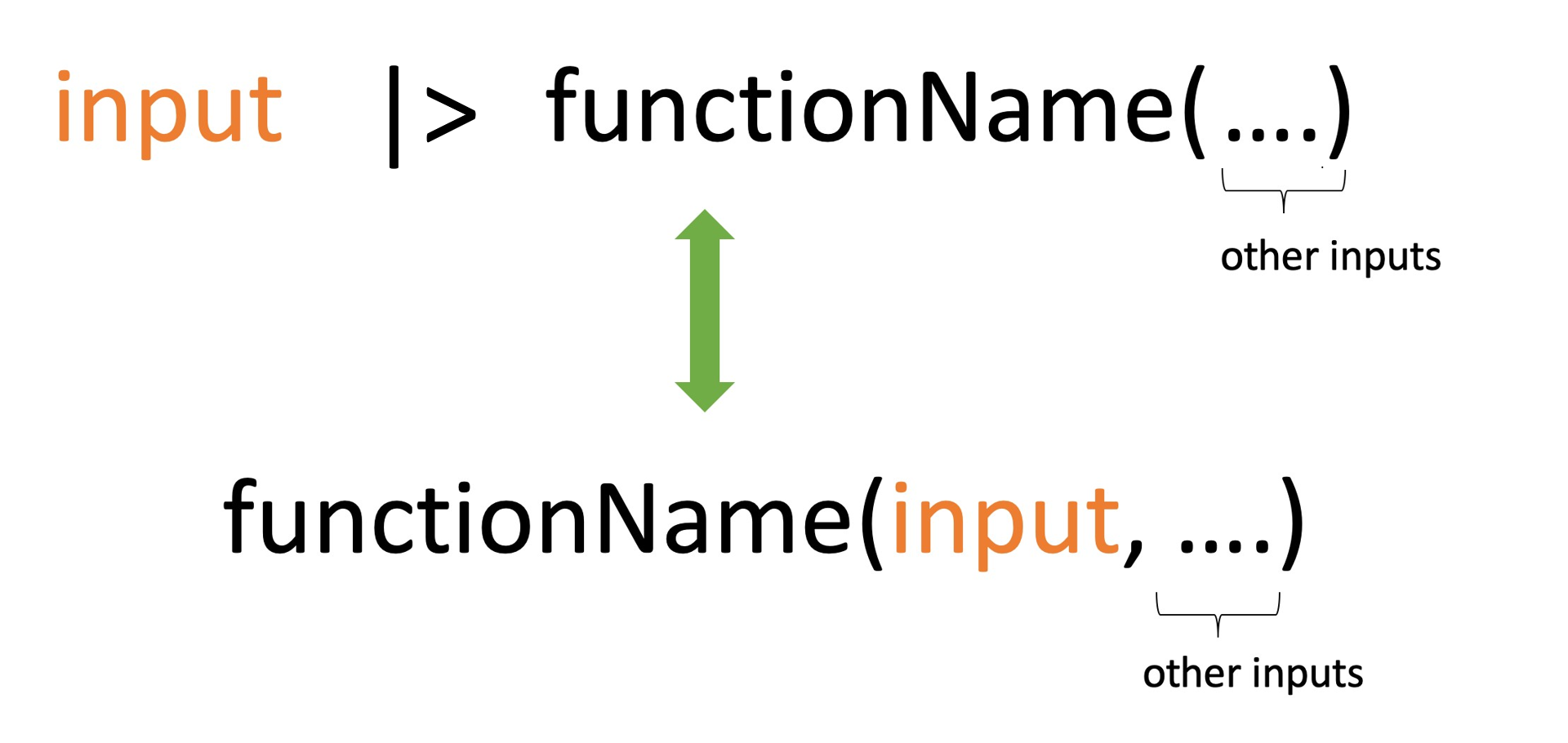
mean(final$Value, na.rm = TRUE) # Calculate the average GDP value

[1] 3506.971

2.7 Pipe operator (|>)

• The pipe operator (|>) in the base R package helps improve the readability of your code.

• It takes the output of one function and passes it directly into another function as an argument, making the steps in your data analysis more connected.

• Instead of using nested function calls like function(first_input, other_inputs), you can write the same command in a simpler format: first_input |> function(other_inputs).

Pipe Operator

• Therefore, using the pipe operator allows you to chain multiple operations together in a way that is easier to read and understand compared to nested function calls.

# Nested function call
mean(final$Value, na.rm = TRUE)

[1] 3506.971

# Using pipe operator) 
final$Value |> mean(na.rm=TRUE)

[1] 3506.971