10  Data Visualization

10.1 Data

The Palmer penguins dataset was introduced by Allison Horst, Alison Hill, and Kristen Gorman provide a great dataset for data exploration and visualization, as an alternative to iris. It was first introduced as an R package. The released version of palmerpenguins can be instaalled from CRAN with:

R Installation install.packages("palmerpenguins")

Using palmerpenguins python package you can easily load the Palmer penguins into your python environment.

Python Installation pip install palmerpenguins

The palmerpenguins package contains two datasets : penguins and penguins_raw. penguins is a simplified version of the penguins_raw data.

10.2 R

Load data

# Load Palmer Archipelago (Antarctica) Penguin Data
library(palmerpenguins)
# Return the first part of the dataset
head(penguins)

# A tibble: 6 × 8
  species island    bill_length_mm bill_depth_mm flipper_l…¹ body_…² sex    year
  <fct>   <fct>              <dbl>         <dbl>       <int>   <int> <fct> <int>
1 Adelie  Torgersen           39.1          18.7         181    3750 male   2007
2 Adelie  Torgersen           39.5          17.4         186    3800 fema…  2007
3 Adelie  Torgersen           40.3          18           195    3250 fema…  2007
4 Adelie  Torgersen           NA            NA            NA      NA <NA>   2007
5 Adelie  Torgersen           36.7          19.3         193    3450 fema…  2007
6 Adelie  Torgersen           39.3          20.6         190    3650 male   2007
# … with abbreviated variable names ¹​flipper_length_mm, ²​body_mass_g

# Retrieve column names
colnames(penguins)

[1] "species"           "island"            "bill_length_mm"   
[4] "bill_depth_mm"     "flipper_length_mm" "body_mass_g"      
[7] "sex"               "year"             

10.2.1 base R package

# Define color for each of the 3 penguine species
colors <- c("#00AFBB", "#E7B800", "#FC4E07")
colors <- colors[as.numeric(penguins$species)]

# Define shapes
shapes = c(16, 17, 18) 
shapes <- shapes[as.numeric(penguins$species)]

plot(x = penguins$flipper_length_mm,
          y = penguins$body_mass_g,
          col = colors,
          pch = shapes,
          xlab = "Flipper Length",
          ylab = "Body Mass" )

10.2.2 gggplot2 Package

ggplot2 is an R package dedicated to data visualization which is based on The Grammar of Graphics (Wilkinson 2012).

#load ggplot2 package to make statistical graphics
library(ggplot2)
p <- ggplot(penguins) +
  geom_point( aes(x = flipper_length_mm,
                  y = body_mass_g,
                  color = species,
                  shape = species)) +
  xlab("Flipper Length")+
  ylab("Body Mass")

print(p)

10.2.3 plotly R package for interactive data visualization

Interactive visualization focuses on graphic representations of data that improve the way we interact with information

plotly is an R package for creating interactive web-based graphs via the open source JavaScript graphing library plotly.js.

library(plotly)
p <- ggplot(penguins) +
  geom_point( aes(x = flipper_length_mm,
                  y = body_mass_g,
                  color = species,
                  shape = species)) +
  xlab("Flipper Length")+
  ylab("Body Mass")

# The function ggplotly converts a ggplot2::ggplot() object to a plotly object.
plotly::ggplotly(p)

Method 2

library(plotly)
fig <- plot_ly(penguins, 
               x = ~flipper_length_mm,
               y = ~body_mass_g, 
               color = ~species,
               symbol = ~species,
               type = "scatter")
fig

10.3 Python

Load data

#load functions in palmerpenguins package
from palmerpenguins import load_penguins
penguins = load_penguins()
# Return the first part of the dataset
penguins.head()
# Retrieve column names
list(penguins.columns)

10.3.1 Matplotlib package

Matplotlib is mainly deployed for basic plotting. Visualization using Matplotlib generally consists of bars, pies, lines, scatter plots and so on.

# Import matplotlib to make statistical graphics. 
# By convention, it is imported with the shorthand sns.
import matplotlib.pyplot as plt

colors = {'Adelie':'blue', 'Gentoo':'orange', 'Chinstrap':'green'}
plt.scatter(penguins.flipper_length_mm,
penguins.body_mass_g, 
c= penguins.species.apply(lambda x: colors[x]))
plt.xlabel('Flipper Length')
plt.ylabel('Body Mass')

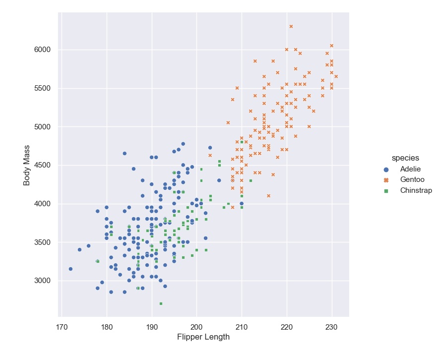
10.3.2 seaborn Package

Seaborn is an easy-to-use high level statistical plotting library which provides a variety of visualization patterns. It uses fewer syntax and has easily interesting default themes.

It tries to provide a ‘grammar of graphics’ style way to create plots but in a pythonic style without getting the exact syntax from ggplot as in plotnine.

Introduction to Seaborn

# Import seaborn to make statistical graphics. 
# By convention, it is imported with the shorthand sns.
import seaborn as sns 
#load functions in palmerpenguins package
from palmerpenguins import load_penguins
penguins = load_penguins()

# Apply the default theme
sns.set_theme()
# sns.set_style('whitegrid')
p = sns.relplot(x = 'flipper_length_mm',
            y ='body_mass_g',
            hue = 'species',
            style = 'species',
            data = penguins)
p.set_xlabels('Flipper Length')
p.set_ylabels('Body Mass')   

The function relplot() is named that way because it is designed to visualize many different statistical relationships. The relplot() function has a convenient kind parameter that lets you easily switch to this alternate representation: scatterplot() with kind="scatter"; the default and lineplot() with kind="line".

10.3.3 plotnine package

https://pypi.org/project/plotnine/

plotnine is an implementation of a grammar of graphics in Python, it is based on ggplot2. The grammar allows users to compose plots by explicitly mapping data to the visual objects that make up the plot.

Plotting with a grammar is powerful, it makes custom (and otherwise complex) plots are easy to think about and then create, while the simple plots remain simple.

NOTE: R vs Python Syntax

Unlike in R, now all the variables must be enclosed by single quotes

from plotnine import *
# unlike in R, now all the variables must be enclosed by single quotes
(ggplot(penguins) +
  geom_point(aes(x = 'flipper_length_mm',
                  y = 'body_mass_g',
                  color = 'species',
                  shape = 'species')) +
  xlab("Flipper Length")+
  ylab("Body Mass"))

10.3.4 plotly Python library for interactive data visualization

The plotly.express (Plotly Express or PX) module contains functions that can create entire figures at once. It is usually imported as px. Plotly Express is a built-in part of the plotly library.

import plotly.express as px

fig = px.scatter(penguins,
                 x="flipper_length_mm",
                 y="body_mass_g",
                 color= "species",
                 symbol= "species",
                 labels=dict(flipper_length_mm="Flipper Length",
                             body_mass_g="Body Mass"))
fig.show()

Wilkinson, Leland. 2012. “The Grammar of Graphics.” In Handbook of Computational Statistics, 375–414. Springer.